── Attaching core tidyverse packages ─────── tidyverse 2.0.0 ──
✔ dplyr     1.1.4     ✔ readr     2.1.6
✔ forcats   1.0.1     ✔ stringr   1.6.0
✔ ggplot2   4.0.1     ✔ tibble    3.3.0
✔ lubridate 1.9.4     ✔ tidyr     1.3.2
✔ purrr     1.2.0
── Conflicts ───────────────────────── tidyverse_conflicts() ──
✖ dplyr::filter() masks stats::filter()
✖ dplyr::lag()    masks stats::lag()
ℹ Use the conflicted package to force all conflicts to become errors1 Prediction vs Causation
Ordinary Least Squares (OLS)
In Econometrics, you studied how to find a line of best fit to describe the relationship between two or more variables using the method of least-squares. That model is:
\[y_i = \beta_0 + \beta_1 x_i + u_i\]
Where:
- \(y_i\) is the dependent variable: it’s the variable you’re trying to model.
- \(x_i\) is the explanatory variable: it’s the variable you’re hoping explains some of the variation in your dependent variable.
- \(\beta_0\) is the y-intercept of the line of best fit,
- and \(\beta_1\) is the slope: its interpretation is that: when \(x\) increases by 1 unit, \(y\) is expected to increase by \(\beta_1\) units. If you’re interpreting the model causally, you’d say that \(\beta_1\) is the effect of \(x\) on \(y\).
The line of best fit is just a statistical relationship describing the nature of the correlation between two variables. Econometrics is focused on the causal inference problem: when is it true that correlation implies causation?
Machine learning, on the other hand, is focused on the prediction problem: instead of trying to understanding why something happens, can we do a good job of predicting what will happen?
This distinction between causal inference and prediction is subtle, but it is one of the most important ideas in this course. The same model can be used to answer two completely different questions: one about changing the world (causal inference), and one about forecasting the world (prediction). Confusing the two can lead to misleading conclusions, bad decisions, and poor policy. This classwork is designed to help you clearly separate these goals and start thinking like both an Econometrician and a data scientist.
Causal Inference
Causal inference asks: “What is the effect of \(x\) on \(y\)”?
The goal is to estimate the true \(\beta_1\), and by estimating that, we get at the mechanisms behind variation in the dependent variable.
That lets us answer the question, “What happens if we change \(x\)?” From there, we can make policy decisions that can help make people’s lives better.
Example
Consider the research question: “What is the effect of education on a person’s lifetime earnings?”
If we knew the true causal effect, we could make meaningful decisions like, “should a person go to college? should they go to graduate school?” and, “how much should the government spend to support students and different educational institutions?”
The tricky thing about causal inference is something called the Fundamental Problem of Causal Inference: it’s impossible to observe the same unit (person, firm, country, etc) under both the treatment and the control conditions simultaneously. We can never know exactly how much your education would impact your lifetime earnings, because we can never observe your life both with a degree and without one.
Suppose we conducted an observational study, surveying a large group of people similar to you, half of whom got a college degree and half of whom did not. If we found that the group with a college degree earns $10K more per year on average than the group without a degree, does that mean education caused that increase? Not necessarily.
The reason is called omitted-variable bias. Even if the two groups of people look similar to each other on observables (demographics, family background, location, etc.), they are likely not similar on unobservables (variables that are hard or impossible to measure). In particular: ability, conformity, and conscientiousness tend to be higher among highly educated people. Those variables are also highly correlated with high earnings. So in an observational study, you can never tell whether it’s the education that drives earnings, or if it’s the underlying ability, conformity, and conscientiousness that makes the college-educated group higher earners.
The gold standard for causal inference is to conduct a randomized, controlled experiment to see how one variable effects another. What would that “ideal” experiment look like here? It’s often outrageous: get a large group of people, divide them randomly in half, assigning one to the “treatment” group, and one to the “control” group. Force the treatment group to go to college, and force the control group to not go. Compare earnings after a lifetime.
Of course, it would not be ethical to control people’s life decisions like this. The “ideal experiment” is often not ethical, especially for some of the most interesting research questions. This is where the causal inference toolkit from Econometrics comes in: using instrumental variables, differences in differences, or regression discontinuity to try to get at that causal effect in a more rigorous way than relying on observational studies alone when the randomized, controlled trial is not ethical.
Prediction
Prediction, on the other hand, asks: “Can we forecast \(\hat{y_i} = \beta_0 + \beta_1 x_i\)?”
We care only about the accuracy of the forecast. We don’t need to know why the predictors work. We just need them to work!
Example
Suppose we want to build a model to forecast a stock return. If we can accurately do that, there’s a lot of money to be made! So we don’t want to build the model to figure out why the return might go up or down, we want to build it to be as accurate as possible.
The core challenge of prediction is that even if a model works well in the past, there’s no guarantee it will work in the future. Relationships can change over time, people can adapt to models, and new environments create new patterns. A model might be highly accurate historically, and still fail going forward.
Note: we can use OLS both for prediction and for causation, but if we built it for causation, it may be terrible at prediction. And if we built it for prediction, it might be terrible for causation.
Classwork #1
Each of these research questions could be explored by fitting a linear model with OLS, or another kind of model we’ll learn about in this class. For each:
- Identify the dependent variable
- Identify the explanatory (or predictor) variables
- Identify whether the problem is a causal inference problem or a prediction problem and explain why. (Hint: 3 will be causal inference; 3 will be prediction)
- If the problem is a causal inference problem, explain the omitted variable bias that might exist if you tried to do an observational study to get at the causal effect. Then explain the ideal (but perhaps unethical) experiment.
- If the problem is a prediction problem, explain what predictors may have made for strong predictions in the past, but that may not hold in the future.
Examples
Finance: What will a stock’s return be tomorrow?
- Dependent variable: a stock’s return
- Predictors: past returns, trading activity, market-wide variables, and firm-specific characteristics
- This is a prediction problem. We want to be able to predict a stock’s returns tomorrow (\(\hat{y}\)). It doesn’t matter if predictors cause a stock’s returns to rise or fall, we just want the most accurate prediction possible.
- past returns may have made good predictions in the past, but if the firm’s growth prospects change suddenly, past returns may become a weaker predictor.
Education: Does education effect earnings?
- Dependent variable: a person’s lifetime earnings
- Explanatory variables: education, location, demographics, family background
- This is a causal inference problem. We want to know about the underlying mechanisms that determine a person’s earnings, especially \(\beta_1\) (the effect of education on earnings).
- Ability, conscientiousness, and conformity are all highly correlated with education and earnings and are very difficult to measure, so in any observational study, education will look like a much stronger determinant of earnings than it actually is.
- The ideal (but unethical) experiment would be to get a large group of people, divide them in two randomly, force one group to get a college education and force the other to not get one, and compare differences in lifetime earnings.
- Will deactivating Facebook or Instagram improve a person’s emotional state?
- What is the expected loan repayment behavior of a borrower?
- How do changes in minimum wage laws effect the unemployment rate?
- What is the effect of smoking on lung cancer risk?
- Which job candidates will perform best in a role?
- Which patients are at high risk of heart disease?
Homework #1
Before Thursday, set up your workspace by downloading R, RStudio, and then complete the ⤓ R Install Check. Come to office hours on Wednesday at 12:30 over Zoom if you get stuck.


Setting up your workspace
Laptop
First thing first, you should decide which laptop you’d like to do your programming assignments on. It can be a Mac, Windows, or Linux machine: all are equally good. If you don’t have a laptop to bring to class, consider checking one out at the HUB or either campus library.
Download and Install R
Do this even if you installed R on your computer for a previous class (it will just update for you).
Go here: https://cran.r-project.org/ and follow the instructions to download R for your Linux, Windows, or Mac. You should download the latest release. If you are a Mac user, first check to see whether you have an Apple silicon mac or an older Intel mac (Top left apple symbol > About this mac > Chip will say M1, M2, … or Intel).
Finish the installation by opening the installer and agreeing to the software license agreement. Click through until you have confirmation it was successful.
Mac users: install xquartz: https://www.xquartz.org/.
Having issues with this step? Try doing your downloads at home instead of on campus. The campus wifi can sometimes be too slow, corrupting the files you’re trying to download.
Install RStudio
Now you’ve downloaded the programming language R! The next step is to download the IDE (Integrated Development Environment): the application you’ll open to work with R.
Go here https://posit.co/download/rstudio-desktop/ and scroll until you see 2. Install RStudio. Download RStudio desktop. Mac users will need to drag the RStudio icon into their applications folder.
Install the Tidyverse
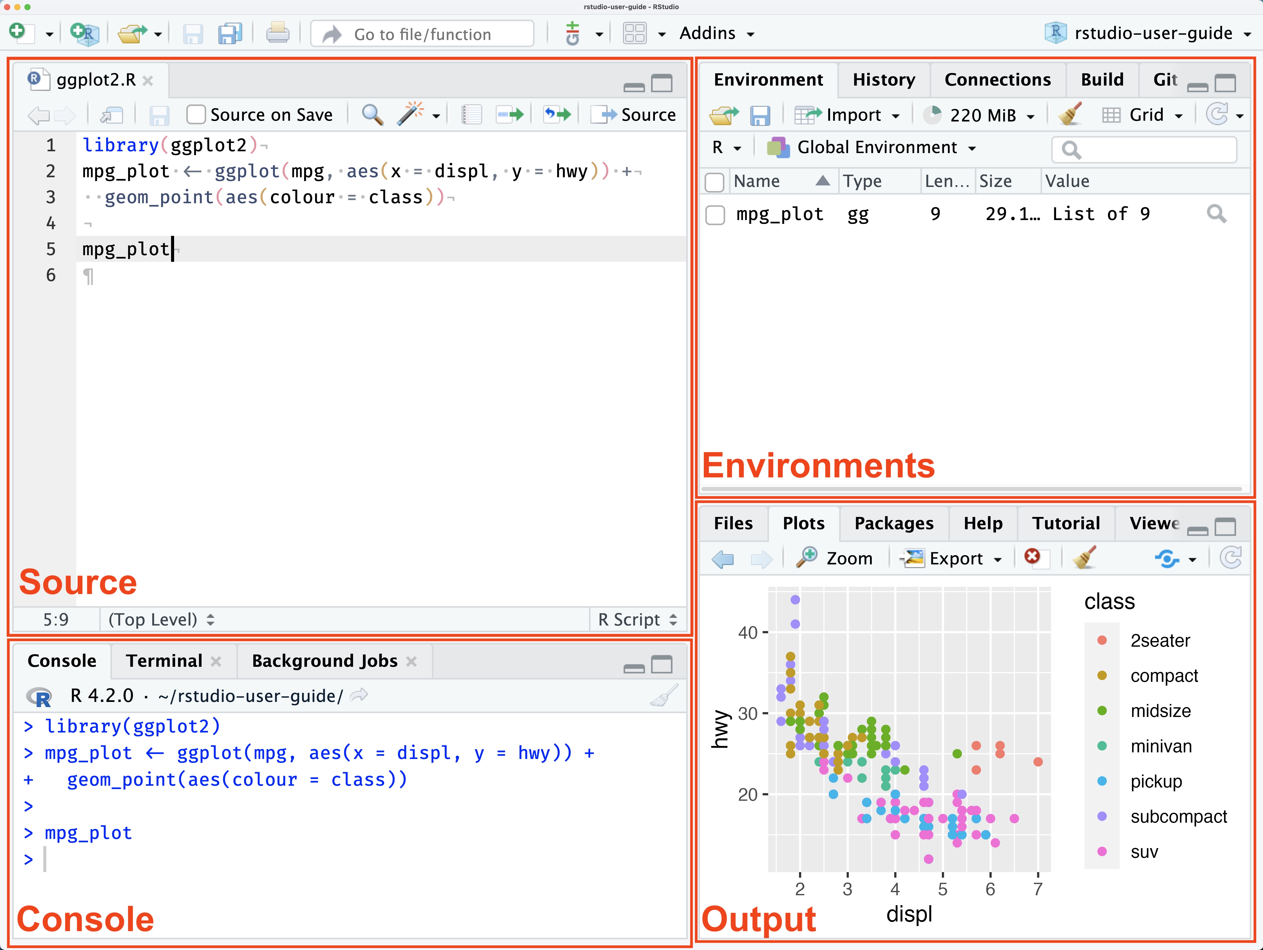
Open up RStudio. You should see 4 panes:
- Source: the document you’re working on. If you’re not working on any document right now, nothing will show up. To start a new R script, go to File > New File > R Script.
- Environments: shows variables you’ve defined in your global environment.
- Console: a scratch pad to run pieces of code and package installations.
- Output: files and rendered plots appear here.
Now locate your console and copy-paste this line of code, then hit enter to install the tidyverse package:
install.packages("tidyverse", dependencies = TRUE)
When it’s done downloading, you’ll see a carrot symbol in your console that indicates it’s ready for more code: >. Let’s check to make sure we’ve successfully downloaded the tidyverse. Run this in your console to attach the tidyverse to your current R session so you can use its functions:
library(tidyverse)
If everything went well, you should see this print:
Install gapminder
You’ll use this package a lot in the first few assignments for this class. Run this in your console:
install.packages("gapminder")
library(gapminder)
Install a few packages we’ll use for plots
install.packages("gganimate", dependencies = TRUE)
install.packages("hexbin")
install.packages("devtools")
Install qelp
qelp (quick help) is an alternative set of beginner friendly help docs I created (with contributions from previous students) for commonly used functions in R and the tidyverse. Once you have the package installed, you can access the help docs from inside RStudio.
install.packages("remotes")
remotes::install_github("cobriant/qelp")
Now run:
?qelp::install.packagesIf everything went right, the help docs I wrote on the function install.packages should pop up in the lower right hand pane. Whenever you want to read the qelp docs on a function, you type ?, qelp, two colons :: which say “I want the help docs on this function which is from the package qelp”, and then the name of the function you’re wondering about.
Submit the R Install Check on Canvas
Now you’ve downloaded R, RStudio, the tidyverse, gapminder, and qelp. To check to make sure you’ve completed all the steps, download this R script: ⤓ R Install Check. Open the R script in RStudio and fill out the questions. When you’re done, compile the document to html (Ctrl/Cmd Shift K) and upload the html document to Canvas under HW #1: R Install Check. That’s all you need to do by Thursday.