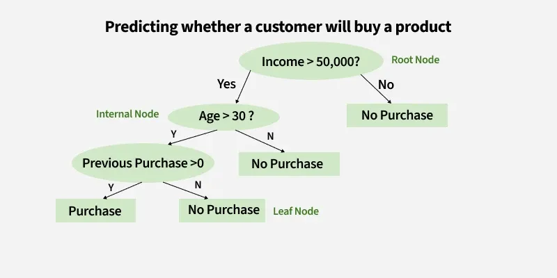
A decision tree is a model that makes predictions by repeatedly splitting data into groups using if-then rules, like “income > $80,000.” It creates a tree-like structure where each branch represents a decision and each leaf gives a prediction. Decision trees are popular because they are easy to interpret and they automatically capture complicated, nonlinear relationships and interactions.
For example:
Question 1: Decision trees are probably the easiest model to interpret, even easier than a linear regression! Interpret the decision tree above: take a person with income $100K/year, age 35, who has not previously purchased the item. Are they predicted to purchase it? Describe the type of people who are most likely to purchase the item.
In this assignment, we’ll work on growing a decision tree by hand. Then we’ll compare our decision tree to the one created with the R package tree.
Part 1: Fitting a Decision Tree
To fit a decision tree, you’ll start at the top (“root node”). There, you’ll consider every possible predictor and every possible cutoff point, one at a time (income < 50K, income < 60K, age < 18, age < 20, age < 22, …).
For each possible split, measure how much that split improves classification purity in the training set, and choose the split that creates the purest child nodes. A popular measure is Gini impurity: \(1 - (p_1^2 + p_2^2)\), where \(p_1\) is the percent of the observations in the first class (approved) and \(p_2\) is the percent of the observations in the second class (denied). For example, if a child node has 50% approved and 50% denied, its Gini would be \(1 - (.5^2 + .5^2) = 0.5\). And if a child node is totally pure and it has 100% approved and 0% denied, its Gini would be \(1 - (1^2 + 0^2) = 0\).
Split the data into two groups based on the root node rule. Then repeat the process separately inside each new node. Stop growing the tree when a stopping rule is reached, like a minimum number of observations in a branch or no meaningful improvement in prediction accuracy. Without a stopping rule, a decision tree will get too deep, memorizing the training data set and overfitting.
Question 2: Calculate the Gini impurity for a group that is 3/4 approved and 1/4 denied.
Let’s practice growing a decision tree by hand with a 100-observation sample of our data.
# A tibble: 100 × 10
   approved income debt_to_income_ratio loan_amount loan_type    loan_purpose
      <dbl>  <dbl>                <dbl>       <dbl> <fct>        <fct>
 1        0    254                   44         655 FHA          Home purchase
 2        1    100                   49         445 Conventional Home purchase
 3        1     15                   41         725 Conventional Home purchase
 4        0    175                   65          35 Conventional Home improveme…
 5        0    207                   55         195 Conventional Cash-out refin…
 6        1    559                   25        1015 Conventional Home purchase
 7        1    114                   46         565 FHA          Home purchase
 8        1    204                   33         465 Conventional Home purchase
 9        0     75                   55          35 Conventional Other
10        0    173                   55         365 FHA          Cash-out refin…
# ℹ 90 more rows
# ℹ 4 more variables: loan_to_value_ratio <dbl>, conforming_loan_limit <fct>,
#   property_value <dbl>, bad_credit <dbl>
Question 3: Let’s work on step 1 of growing the decision tree: taking one variable (income), one possible split (100K/year), and evaluating the Gini impurity of the children. Sketch what the tibble might look like after summarize() and then after the mutate().
split <-100mortgage_small %>%group_by(income < split) %>%summarize(p1 =mean(approved), group_size =n()) %>%# calculate the gini impurity of both childrenmutate(group_size = group_size /sum(group_size),p2 =1- p1,gini =1- (p1^2+ p2^2) ) %>%# the overall impurity of a split is the weighted average of the child ginissummarize(impurity =sum(gini * group_size))
# A tibble: 1 × 1
  impurity
     <dbl>
1    0.400
Question 4: Fill in the blanks to write a helper function evaluate_split that takes any variable and any split value and outputs the impurity of the split.
evaluate_split <-function(________, ________) { mortgage_small %>%group_by({{ var }} < split) %>%summarize(p1 = ________, group_size =n()) %>%# calculate the gini impurity of both childrenmutate(group_size = group_size /sum(group_size),p2 = ________,gini = ________ ) %>%# the overall impurity of a split is the weighted average of the child ginissummarize(impurity =sum(gini * group_size))}
Question 5: Evaluate: what is the best split for income?
Question 6: Now we would look at every other variable and every other possible split to see if there’s a better split we can make at the root node. Let’s evaluate debt_to_income_ratio. What’s the best split here? Is it better to split on income or on debt to income in the root of our decision tree?
After we evaluate all variables and select the best one to form the root node decision rule, we would split the data into two groups, and repeat the process over again for the next node, continuing until we’ve met some stopping criteria. Finally, using a threshold to make predictions at every terminal node. Let’s let tree handle those details.
Part 2: Using tree to Fit a Decision Tree
install.packages("tree")
Question 8: Write code to split mortgage into 80% training (mortgage_train) and 20% test (mortgage_test).
Classification tree:
tree(formula = approved ~ income + debt_to_income_ratio + loan_amount +
    loan_type + loan_purpose + loan_to_value_ratio + conforming_loan_limit +
    property_value + bad_credit, data = mortgage_train %>% mutate(approved = factor(approved)))
Variables actually used in tree construction:
[1] "debt_to_income_ratio" "bad_credit"           "loan_purpose"
[4] "loan_type"
Number of terminal nodes:  6
Residual mean deviance:  0.6565 = 19400 / 29550
Misclassification error rate: 0.1165 = 3443 / 29560
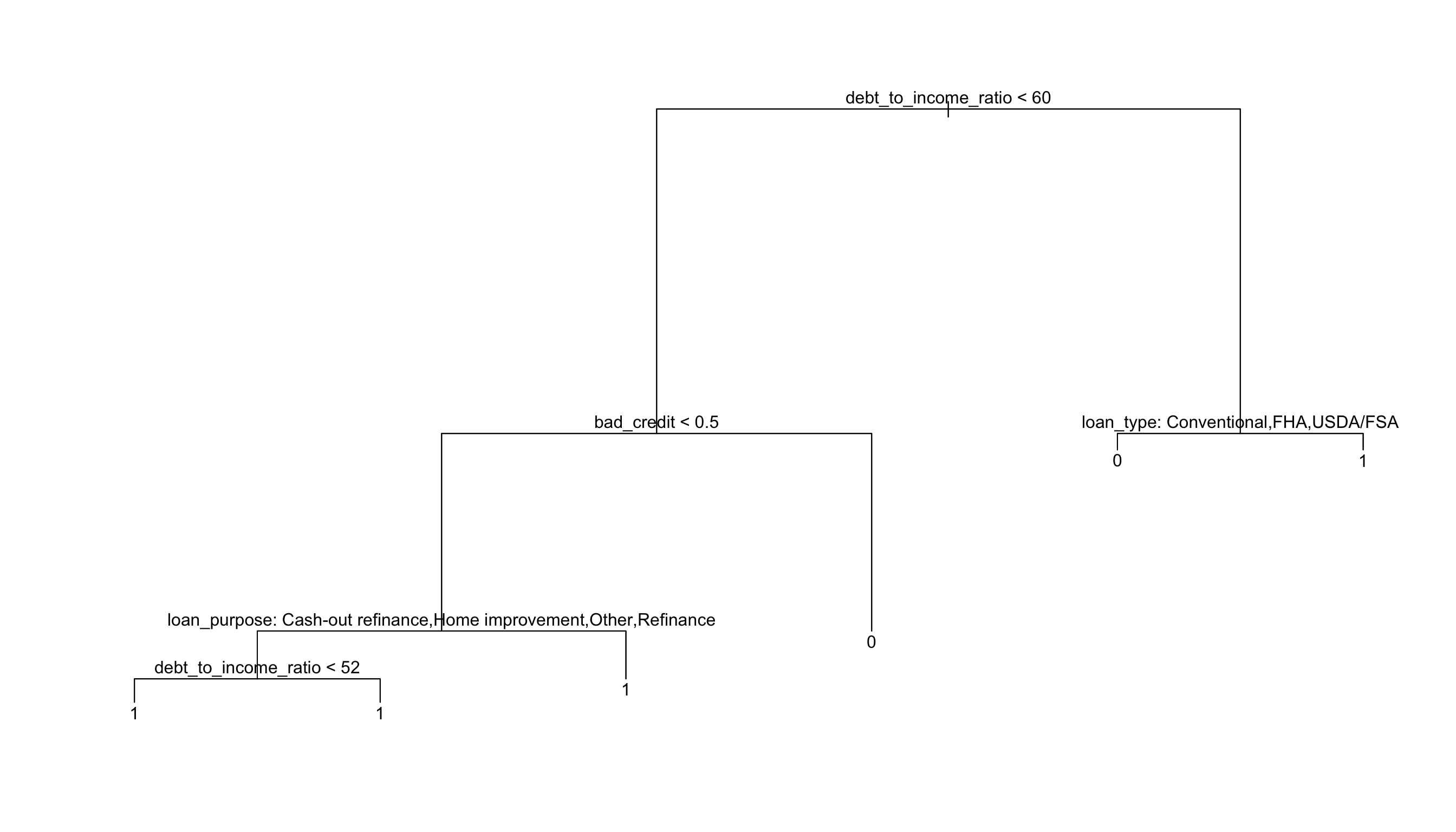
plot(mortgage_tree)text(mortgage_tree, pretty =0)
Question 9: Interpret the mortgage application decision tree: the left hand branches always correspond to “TRUE” and the right hand branches to “FALSE”. What types of people do we predict get approved versus denied? Why are there branches with predictions of 1 on both sides?
Question 10: What is the test accuracy of the decision tree?