Ridge and LASSO on the Mortgage Problem
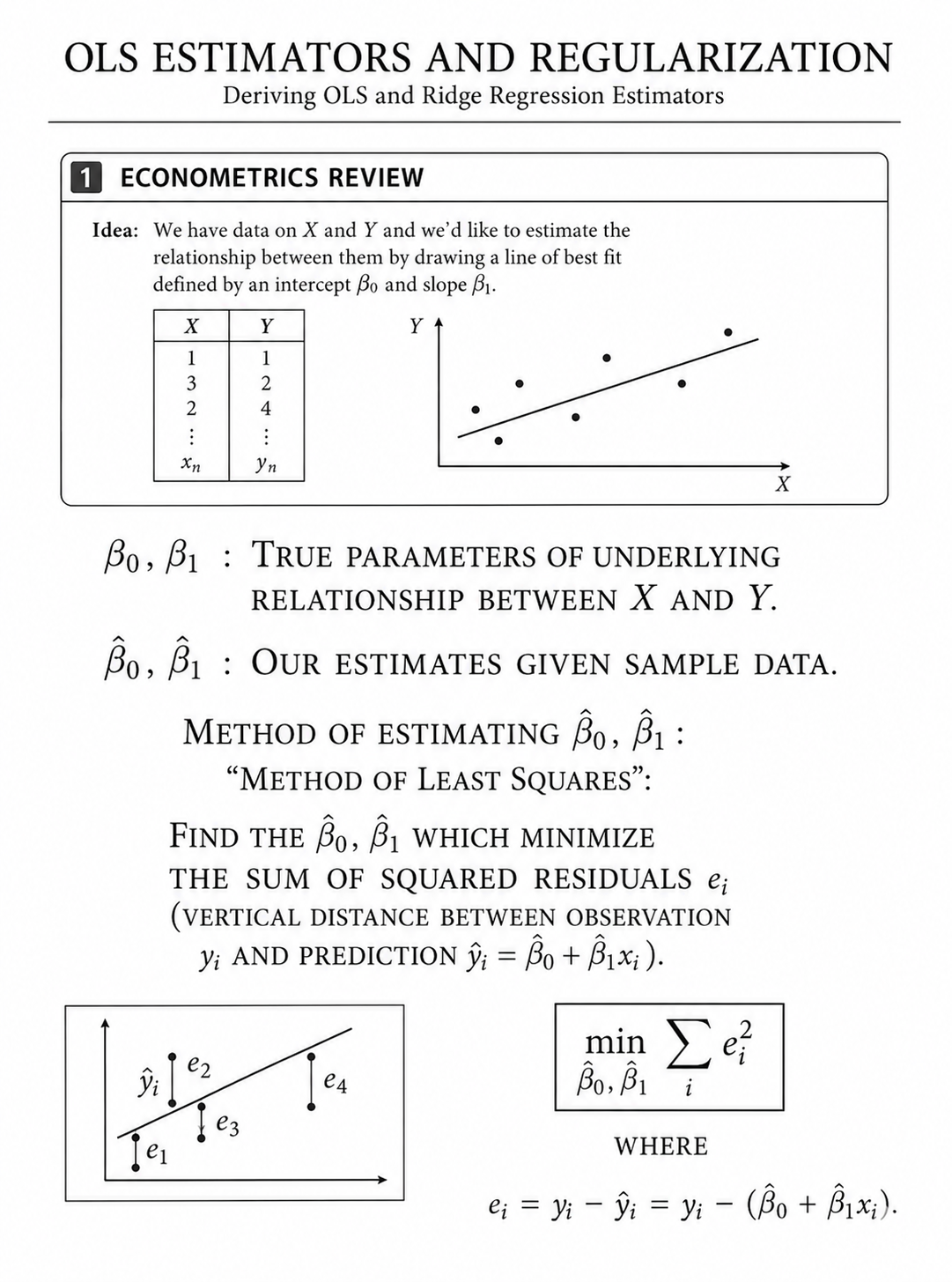
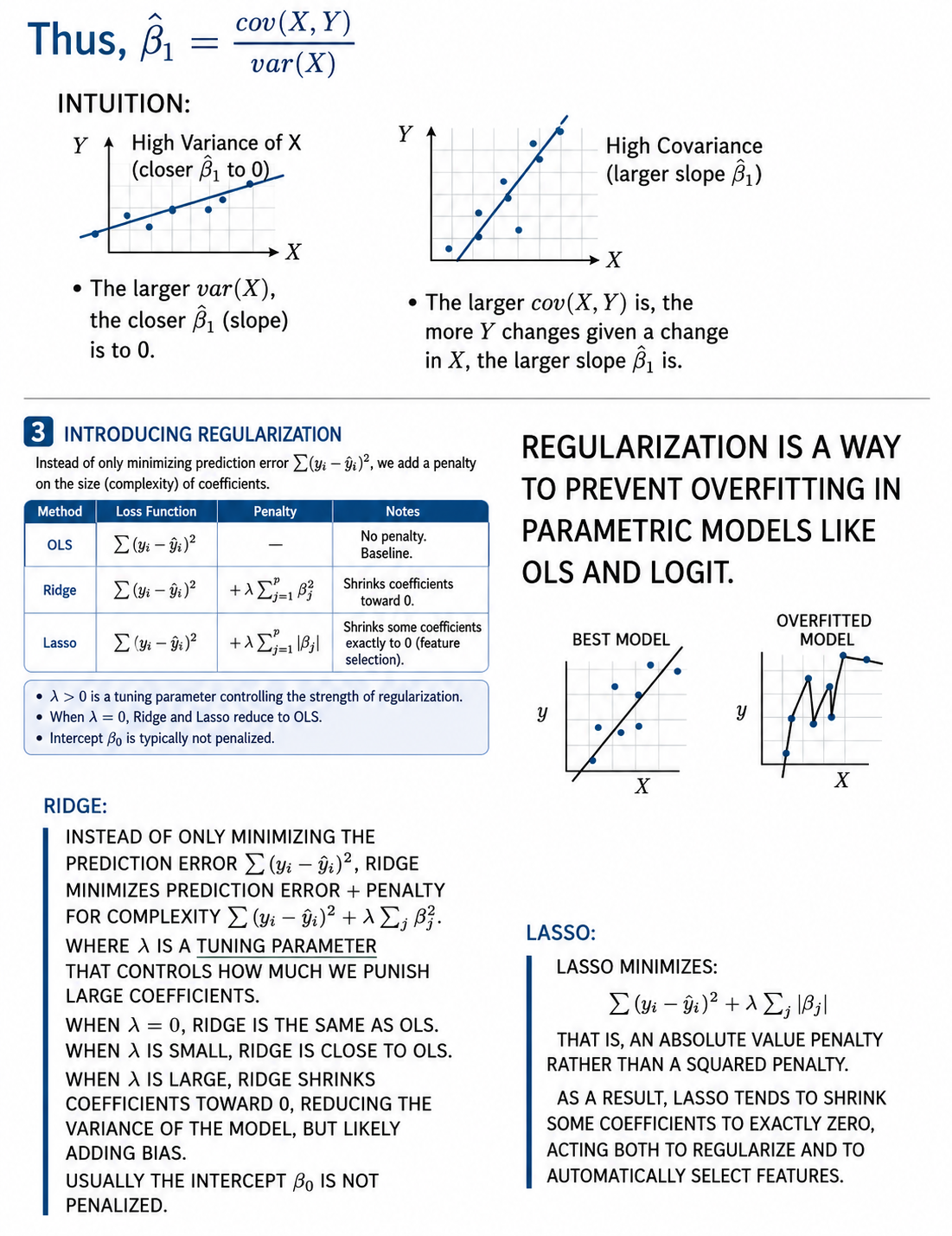
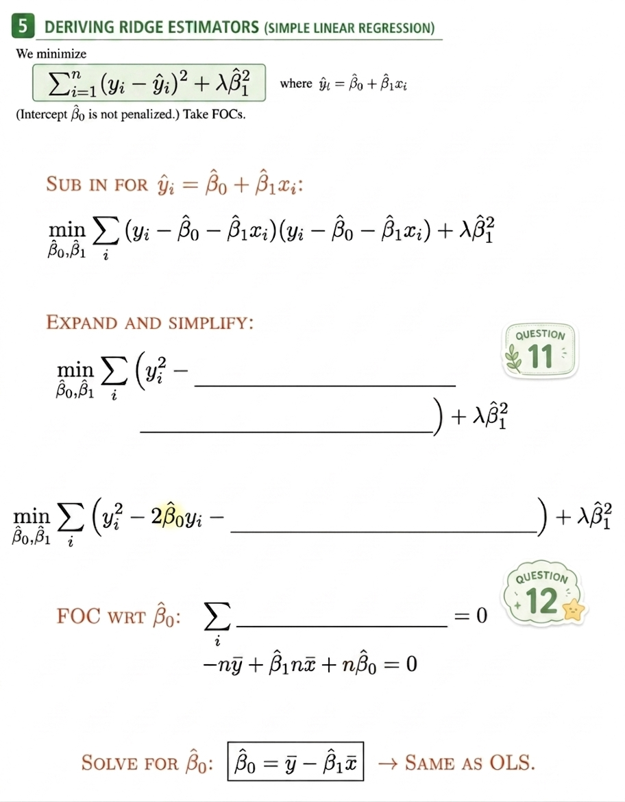
First, showing that \(\hat{\beta}_1 = \frac{cov(x, y)}{var(x)}\) :
%>% summarize (lm_beta1 = cov (approved, income) / var (income)
# A tibble: 1 × 1
  lm_beta1
     <dbl>
1 0.000785
%>% lm (approved ~ income, data = .) %>% :: tidy ()
# A tibble: 2 × 5
  term        estimate std.error statistic   p.value
  <chr>          <dbl>     <dbl>     <dbl>     <dbl>
1 (Intercept) 0.665    0.00437       152.  0
2 income      0.000785 0.0000250      31.5 2.80e-214
# CV AUC for LPM, logit, and KNN %>% select (- race, - ethnicity, - sex, - age) %>% mutate (fold = sample (1 : 5 , size = nrow (.), replace = T)) %>% c (lpm = cross_validate (., "lpm" ),ridge_lpm = cross_validate (., "lpm ridge" ),lasso_lpm = cross_validate (., "lpm LASSO" ),logit = cross_validate (., "logit" ),ridge_logit = cross_validate (., "logit ridge" ),lasso_logit = cross_validate (., "logit LASSO" )# CV AUC: # LPM: ___ # LPM with ridge: ___ # LPM with LASSO: ___ # Logit: ___ # Logit with ridge: ___ # Logit with LASSO: ___
If Ridge or LASSO help our CV AUC a lot, that’s an indicator that our models are overfitted. Is that a problem for us?
Compare Coefficients
Inspect the coefficients for the LPM, LPM with ridge regularization, and LPM with LASSO. Which coefficients shrink or disappear?
<- mortgage %>% select (- race, - ethnicity, - sex, - age)# No regularization <- mortgage %>% lm (approved ~ ., data = .) %>% :: tidy () %>% select (term, ols_estimate = estimate)# Ridge <- cv.glmnet (x = model.matrix (approved ~ ., data = mortgage)[, - 1 ],y = mortgage %>% pull (approved),alpha = 0 , # 0 = ridge; 1 = lasso family = "gaussian" %>% coef (s = "lambda.1se" ) %>% as.matrix () %>% as_tibble (rownames = "term" ) %>% rename (ridge_estimate = 2 )# Lasso <- cv.glmnet (x = model.matrix (approved ~ ., data = mortgage)[, - 1 ],y = mortgage %>% pull (approved),alpha = 1 , # 0 = ridge; 1 = lasso family = "gaussian" %>% coef (s = "lambda.1se" ) %>% as.matrix () %>% as_tibble (rownames = "term" ) %>% rename (lasso_estimate = 2 )# View coefficients from all three: %>% left_join (ridge) %>% left_join (lasso)
# A tibble: 50 × 4
   term                           ols_estimate ridge_estimate lasso_estimate
   <chr>                                 <dbl>          <dbl>          <dbl>
 1 (Intercept)                       -1.68         0.808              0.0842
 2 income                             0.000145    -0.000230           0
 3 debt_to_income_ratio               0.0588       0.00189            0.0440
 4 loan_amount                       -0.00101     -0.00000199         0
 5 loan_typeFHA                       0.0410       0.0622             0.0496
 6 loan_typeUSDA/FSA                 -0.140       -0.155             -0.106
 7 loan_typeVA                        0.101        0.0976             0.102
 8 loan_purposeCash-out refinance    -0.142       -0.106             -0.125
 9 loan_purposeHome improvement      -0.143       -0.111             -0.122
10 loan_purposeOther                 -0.186       -0.150             -0.167
# ℹ 40 more rows
Reflection Questions:
Compare the coefficients across OLS, ridge, and lasso. List the variables whose coefficients remained stable and then those that changed dramatically. Are the coefficients that remained stable the variables that might be less correlated with other explanatory variables?
Did LASSO force any variables to totally disappear? Does it make sense that these variables are not as important to our prediction?
Ridge and LASSO changed many coefficients, but CV AUC barely changed. What does this suggest about interpreting coefficients in predictive models?
Download this assignment
Here’s a link to download this assignment.